Overview of Using Vericut
Vericut enables you to simulate the NC machining process with software files, 3-D models, and functions. Setting up an NC program to be processed by Vericut is similar to setting up an NC program to run on an NC machine tool.
💡 Tip: Try using the general purpose startup files in the \library folder of your Vericut installation to set the simulation environment, and then add your stock models, NC programs, and cutting tools.
See Library Files, also in the Getting Started section of Vericut Help for details.
Requirements for a simulation
Vericut requires three things to simulate the cutting action of an NC program, the same things that are required to machine the actual part on an NC machine tool:
Stock — raw material, or "workpiece" to be machined
NC Program — NC data describing cutting tool positions, machine information, and other data required to operate a machine tool
Cutting tools — shapes and sizes of cutting tools used to machine the workpiece
The items below are optional, however, can aid in the verification effort.
-
Fixture — hardware used to hold the workpiece for machining
-
Designed part — the theoretical perfect machined part
-
Operator instructions — notes about actions required by the machine operator which must be followed in order to successfully machine the part, such as: part setup, clamp/fixture changes, tool changes, etc.
The table below shows the requirements for setting up an NC Program to run on an NC machine tool, and how these requirements are met in Vericut.
| Requirement | NC Machine Tool | Vericut |
|---|---|---|
| Workpiece | Metal, or other stock material | Stock model |
| NC data (Tool positions and NC machine codes) | NC program file(s) G-Code format | NC program file(s) APT-CLS or G-Code format |
| Cutting tools | Cutting tools | Descriptions of cutting tools shape/size |
| Holding fixtures | Clamp/fixture hardware | Clamp/fixture models |
| Designed part | Not available until machined | CAD-designed model, or other design data |
| Operator instructions | Operator instructions | Operator instructions |
Basic Steps for Setting up a Vericut Project
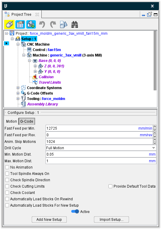
- In the Project Tree, enter the settings for Setup 1.
-
Save the Project (File tab > Save Project)
-
Play Setup 1
 (Play/Start – Stop Options)
 -
Save Setup1.ip (File tab > Save In-Process)
-
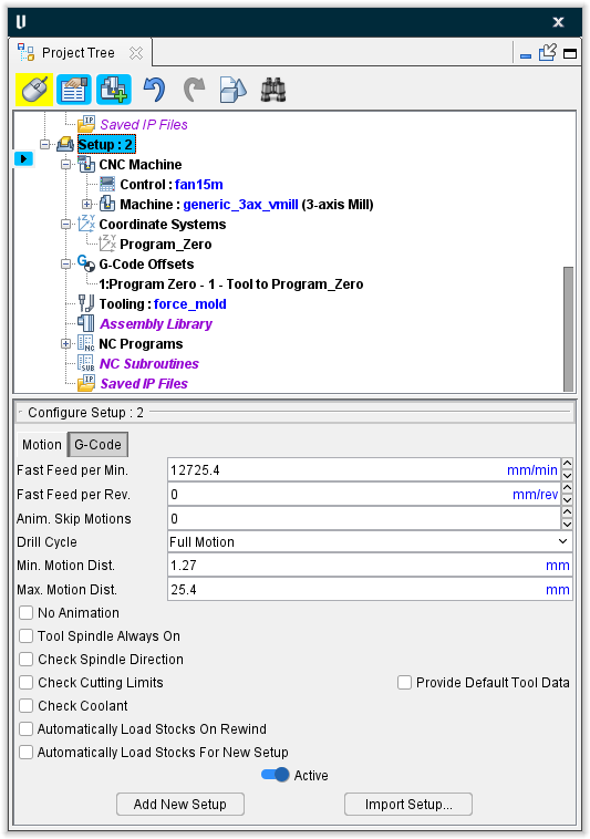
Add or Import Setup 2. (Project tab > Add New Setup) or (Project tab > Import Setup)
-
Single Step to move the Cut Stock to Setup 2.
 (Step/Subroutine Options)
 -
In the Configure Model menu, orient the Cut Stock and then Preserve Stock Transition.
- In the Project Tree, enter the settings for Setup 2.
- Save/Update the Project (File tab > Save Project)
- Play Setup 2 (Play/Start – Stop Options)
- Save Setup2.ip (File tab > Save In-Process)
- Save the final Project. (File tab > Save Project)
Vericut Axes and Coordinate Systems
Vericut uses the axes and coordinate systems described below to: define and relate components and their models, define NC machines, and orient NC programs for proper cutting. Axes are created by Vericut and are stored in the Preferences file.
Coordinate Systems (CSYS) are user defined and are stored in the "setup". Using Project tab > Axes, to display the View Axes window, enables you to display symbols representing these axes and coordinate systems to see how they relate to each other.
Once displayed, axes and coordinate system symbols remain displayed until turned off via selecting the item in the View Axes window again. Solid lines indicate that an axis is parallel or pointing out of the screen. Dashed lines indicate that an axis is pointing into the screen.
See View Axes window, in the View tab section of Vericut Library for additional information.
AXES
Component axes — (XcYcZc) represent the coordinate system of an individual component. Each component has its own coordinate system. Components are defined and connected to other components via the features on the Project Tree, Configure Component menu (ref. Configure Component menu in the Project Tree section of Vericut Help). You can display the axes of a selected component via Project tab > Axes: Component.
Model axes — (XmYmZm) represent the coordinate system of an individual model. Each model has its own local coordinate system. Models are associated with components to provide 3-D properties. Models are defined and associated with components via the features on the Project Tree, Configure Model menu (ref. Configure Model menu in the Project Tree section of Vericut Help). You can display the axes of a selected model via Project tab > Axes: Model.
Machine axes — (XmchYmchZmch) represent Vericut's "base" or "world" coordinate system. Applicable mainly to views displaying an NC machine, this coordinate system is referenced when defining NC machines and tables for use with the machines. X-caliper measurements in a machine view are relative to this coordinate system. You can display these axes via Project tab > Axes: Machine Origin.
Workpiece axes — (XwpYwpZwp) represent the coordinate system to which Stock, Fixture, and Design components are connected. This coordinate system only applies to workpiece views, and takes on a slightly different meaning, depending on if an NC machine is used in the simulation.
-
In a simulation where a machine is defined, such as when processing G-Code files, the workpiece coordinate origin is the origin the machine component responsible for carrying the Stock, Fixture, and Design components.
-
In a simulation where a machine is NOT defined, such as when processing APT-CLS files, the workpiece coordinate origin is the origin of the non-moving "Base" component to which Stock, Fixture, and Design components are connected. In previous Vericut versions, this was known as the "World coordinate system" (XwYwZw axes).
You can display these axes via Project tab > Axes: Workpiece Origin.
Tool Tip axes — (XtooltipYtooltipZtooltip) The Tool Tip axes represent where the tool tip (the Vericut control point) of the "active" tool would be located, relative to the "active" stock, if all linear axes were positioned at zero. You can display these axes via Project tab > Axes: Tool Tip.
Driven Point Zero axes — (XdrivenpointYdrivenpointZdrivenpoint) The Driven Point Zero axes represent where the driven point of the "active" tool would be located, relative to the "active" stock, if all linear axes were positioned at zero. The display is based on the actual Machine/Control configuration and therefore may be displayed as a right hand axis, a left hand axis or possibly even a non-orthogonal axis. The Driven Point Zero axes are displayed in Workpiece and Machine views. You can display these axes via Project tab > Axes: Driven Point Zero.
See View Axes window, in the View tab section of Vericut Help for additional information.
COORDINATE SYSTEMS (CSYS)
Coordinate Systems — (Xcsys name Ycsys name Zcsys name) Coordinate systems are defined by the user via the features on the Project Tree, Configure Coordinate System menu. See Configure Coordinate System menu in the Project Tree section of Vericut Help for additional information.
Designate the "active" coordinate system by right-clicking on a coordinate system in the Project Tree and selecting "Active" from the menu that displays. You can also designate the "active" coordinate system using Project tab > Active Coordinate System and then selecting the desired coordinate system from the pull-down list.
The "active" coordinate system applies to X-Caliper measurements, Section plane values, and tool path motions (except when a coordinate system has been associated with an NC program in the Project Tree (ref. NC Program File under NC Programs Branch in the Project Tree section of Vericut Help)).
A user-defined coordinate system is typically used to relocate an NC Program for proper relationship to the workpiece, but you can also activate different coordinate systems for defining section planes or gathering measurement data.
You can display representations of these coordinate systems via Project tab > Axes: Coordinate Systems features. Individual coordinate systems can be toggled On/Off and display colors defined using the features in the View Axes window.
See View Axes window, in the View tab section of Vericut Help for additional information.
Using Mathematical Equations/Expressions in Vericut
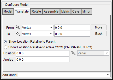
Equations/expressions can be used in any data field within Vericut where a numeric value is expected. They can be used for "single value" data fields like the Increment value in the Project Tree Configure Model menu illustration below. The can also be used for "triplet value" data fields like the Position values shown in the illustration. When using triplet value data fields separate the equations/values with a blank space.
Examples:
| Equation / Expression | Value as interpreted by Vericut |
|---|---|
| sqrt(sqr(4.5) + sqr(2.3) + sqr(6.5)) | 8.2334 |
| trunc(543.6544) | 543 |
| ec | 2.718282 |
| ec ** (1.2 * log(1.256)) | 1.3145 |
| a = acos(⅗) | 53.1301 |
| b = asin(⅘) | 53.1301 |
| c = 2 * 3 * 5 | 30 |
| sqrt(sqr(3) + sqr(5) - c * cos(a)) | 4 |
| pi | 3.141593 |
The following mathematical functions/features are available for use within equations/expressions in Vericut:
| MATHEMATICAL FUNCTION/FEATURE | DESCRIPTION |
|---|---|
| + | Addition |
| - | Subtraction |
| * | Multiplication |
| / | Division |
| mod | Modulus |
| ^ or ** | Exponentiation |
| (, [ or { | Left Parenthesis |
| ), ] or } | Right Parenthesis |
| sqr or square | Square |
| sqrt or root | Square Root |
| abs | Absolute Value |
| int or trunc | Integer Part |
| frac | Fractional Part |
| nint | Nearest Integer |
| pi | Ratio of circle circumference to diameter |
| sin | Sine (argument in degrees) |
| cos | Cosine (argument in degrees) |
| tan | Tangent (argument in degrees) |
| asin | Inverse Sine (result in degrees) |
| acos | Inverse Cosine (result in degrees) |
| atan | Inverse Tangent (result in degrees) |
| atan2(y:x) | Inverse Tangent (result in degrees) |
| sinh | Hyperbolic Sine |
| cosh | Hyperbolic Cosine |
| tanh | Hyperbolic Tangent |
| e or ec | Euler's Constant |
| log | Natural Logarithm |
| analog or exp | Natural Anti-Logarithm |
| log10 | Base 10 Logarithm |
| alog10 | Base 10 Anti-Logarithm |
| fac | Factorial |