Graphs
Location:
Optimize tab > Graphs
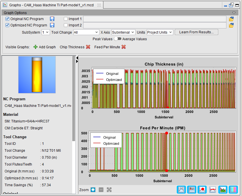
Graphs window
The Graphs window provides a graphical representation of the data generated by Optimizer. This window can be opened at any time, even while the simulation is still running and it will live update as the simulation is processed. Multiple setup files can be set in when Force CSV files are automatically saved to multiple files.
 (Collapse) — Hides the Display Options features so that only the data display and the graphs themselves are visible.
📝 NOTE: The line between the Data Display and the graphs is movable. You can choose how much horizontal space it takes up by clicking and dragging with the mouse to adjust.
Original NC Program — Toggles the display of the Force analysis results of the original NC program. The save icon enables you to save the Force data in a .csv file format.
Optimized NC Program — Toggles the display of the Force analysis results of the optimized NC program. The save icon enables you to save the Force data in a .csv file format. This file will only be available if Force was run in “Optimize” mode.
Import 1 — Toggles the display of the Force analysis results of an imported .csv file saved previously. Click on the  (Browse) icon and use the Set Data Directory file selection window to specify the \path\filename. Previous File and Next File arrows appear next to the Browse icon to more easily navigate multi file setups.
Import 2 — Toggles the display of the Force analysis results of an imported .csv file saved previously. Click on the (Browse) icon and use the Set Data Directory file selection window to specify the \path\filename. Previous File and Next File arrows appear next to the Browse icon to more easily navigate multi file setups.
Any combination of the four files can be shown at once.
SubSystem — Use this dropdown menu to select which subsystem the selected graph or graphs will display data for.
Tool Change — Use this dropdown menu to select which tool the selected graph or graphs will display data for. By default, the Tool Change selects All tools to display until you select a specific tool.
📝 NOTE: Tool Change dropdown is only enabled when it is determined that all of the files being displayed are related to one another or come from the same NC program.
X Axis — Use this dropdown menu to select whether the X Axis will be plotted vs Time, vs Subinterval, or Sorted. Plotting vs Subinterval allows for a direct comparison of cuts between different files. The X Axis “Sorted” graphs view sorts recorded values for the each charted settings in ascending order.
📝 NOTE: The Subinterval option is only used for file comparison and will not be an available option if the files being displayed are from different NC programs.
Units — Use this dropdown menu to select whether the graphs will display measurements in Project Units, Inch, or in Millimeter formats. Project Units option defaults to whatever units the current project is using.
Learn From Results — This button opens the Learn From Results window, enabling you to specify settings to use for optimization.
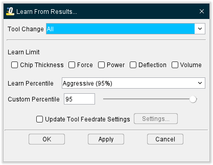
Tool Change — use to select sections of the graph to view specific tool changes.
Learn Limit — Toggle these features on (checked) to use them to limit which results are generated. Features to toggle include Chip Thickness, Force, Power, Deflection, and Volume.
Learn Percentile — Use to set the percentage along the NC Programmed graphed values for Max Chip, Force, Power, and/or Deflection.
📝 NOTE: this is not the percentage of max chip, max force, max power or max deflection.
💡 Tip: Use Force Graphs x Axis sorted to see what the percentile value this setting will return.
Custom Percentile — use to set a specific amount. This amount can either be entered manually in the text field or by using the slider.
Update Tool Feedrate Settings — toggle this feature on (checked) to gain access to the Settings... feature.
Settings... — opens the Tool Feedrate Settings window, enabling you to make changes to various feedrates.
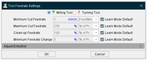
Tool toggle — choose between Milling Tool, Hole Making Tool, and Turning Tool options.
Minimum Feedrate Change — specifies the minimum change from the current optimized feed rate that will cause a new optimized feed rate to be output. This feature controls the quantity of feed rates output to the optimized NC program file. A small value causes more optimized feed rates to be output than when a larger value is entered. Default is 100% of Max Feed Rate for Direction Change.
Minimum Cut Feedrate — specifies the minimum optimized feed rates that can be output when removing material. Default is the same as Minimum Feedrate Change.
Maximum Cut Feedrate — specifies the maximum optimized feed rates that can be output when removing material. Default is 150% of Max Feed Rate(90% of Clean Up Feedrate).
Air Cut Feedrate — this option is useful for reducing time of proven NC programs, without affecting cutting feed rates and resulting surface finishes. When the checkbox is cleared, this feature controls the feed rate used by all other optimization methods to optimize air cuts. Default is 100% of Max Feed Rate.
Clean-up Feedrate — feedrate used when the tool is adjacent to, but not removing material. This condition is commonly referred to as a "spring pass". Default is 50% of Max Feed Rate.
OK — confirms the settings and closes the window.
Cancel — closes the window without confirming settings.
OK — Applies the settings and closes the window.
Apply — Applies the settings without closing the window.
Cancel — Closes the window without applying the settings.
Peak Values / Average Values — This switch allows the user to toggle between viewing the peak or average Force values recorded. It is toggled to view average values by default. It becomes disabled (grayed out) during the simulation or if ‘Record Average Force Conditions’ is turned off in the graph preferences and settings.
Peak Values: Each subinterval datapoint is created from the maximum value found throughout the dynamic milling data for that subinterval. Peak values are useful for optimization because they produce the most conservative result (i.e., lowest feedrates). Comparing optimization limits against peak values ensures that at no point during the cutting process the limit is violated. Currently, peak values are used exclusively for the optimization process. Average values are strictly for analysis purposes.
Average Values: Each subinterval datapoint is created from the time-averaged value of the dynamic milling data for that subinterval. Average values, by definition, will be strictly smaller than peak values. These values are often more likely to line up with predicted values from other software/calculators/databases, etc. They are also often more likely to line up with the readings of on-machine measurements such as spindle torque/power meters which physically have a somewhat “averaged” sampling of the cutting dynamics.
Visible Graphs
Add Graph — Selecting this option opens the Visible Graphs window, enabling you to toggle on (checked) or off (not checked) which graphs will be displayed. You can also click the Clear All button to toggle all graphs off.
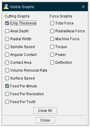
These names will also appear next to Visible Graphs when they are active. They can be removed by clicking the red x next to their name without having to return to the Visible Graphs window.

The following options are current available:
Cutting Graphs:
Force Graphs:
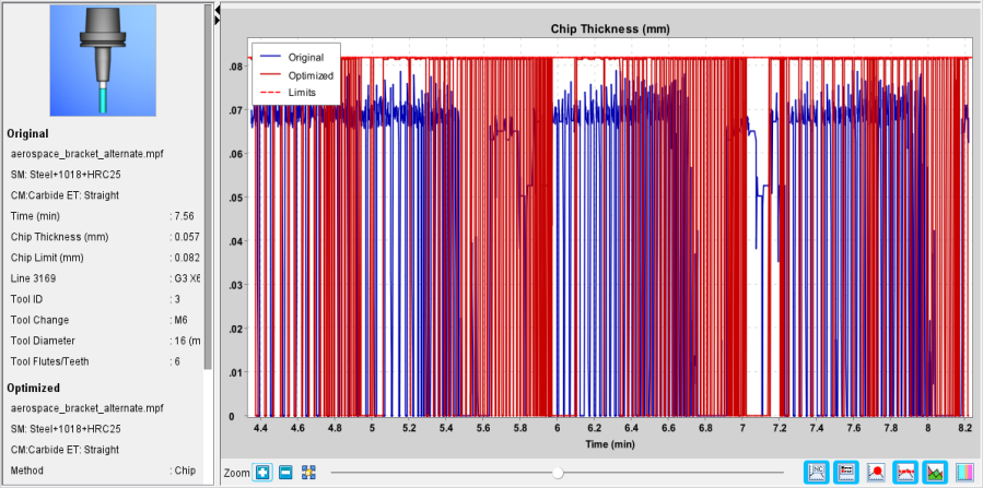
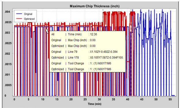
Chip Thickness — This graph displays the maximum chip thickness, adjusted for chip thinning effects, across the entire tool engagement.
Milling — The maximum value of the uncut chip thickness anywhere in material contact for the associated subinterval of motion. The concept of chip thickness used here is the actual physical chip thickness seen by a local portion of an individual cutting edge in an instant in time. This means it inherently includes all chip thinning effects. The value returned is the maximum of all these local values throughout a rotation of the tool. Except for special cases like occur in 5-axis kinematics, this value will always range from 0 (no contact) to a maximum of the Feed Per Tooth value.
Turning — The maximum value of the uncut chip thickness anywhere in material contact for the associated subinterval of motion. The concept of chip thickness used here is the actual physical chip thickness seen by a local portion of an individual cutting edge in an instant in time. This means it inherently includes all chip thinning effects. The value returned is the maximum of all these local values. Except for special cases like 5-axis kinematics, this value will always range from 0 (no contact) to a maximum of the Feed Per Revolution value.
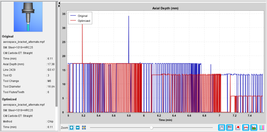
Axial Depth — This graph displays the depth of cut.
Milling — The distance in the axial direction of the tool from the lowest to the highest point of material contact on the tool for the associated subinterval of motion. Stated simply, this is length of contact on the tool in the axial direction. Note that this is NOT the same thing as the distance from the tool tip to the highest point of contact unless the lowest point of contact is at the bottom of the tool.
Turning — The distance in the axial direction of the turning plane from the lowest to the highest point of material contact on the tool for the associated subinterval of motion. Stated simply, this is length of contact on the tool (e.g., insert) in the axial direction.
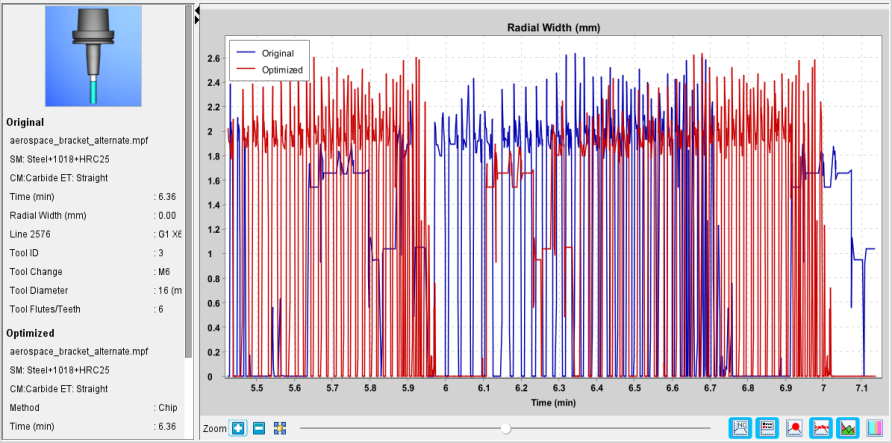
Radial Width — This graph displays the width of cut.
Milling — The maximum extent of material contact on the tool in the radial direction when projected in the direction of motion. For simple horizontal motions with simple material contact, the expected classical definition of radial width will be returned. For non-horizontal motions and those with complex material contact (e.g., multiple discrete contact areas, etc.) the definition of radial width is ambiguous and inexact. Vertical motions return 0. The range of this value is from 0 to the maximum tool diameter.
Turning — The distance in the radial direction of the turn plane from the lowest to the highest point of material contact on the tool for the associated subinterval of motion. Stated simply, this is length of contact on the tool (e.g., insert) in the radial direction.
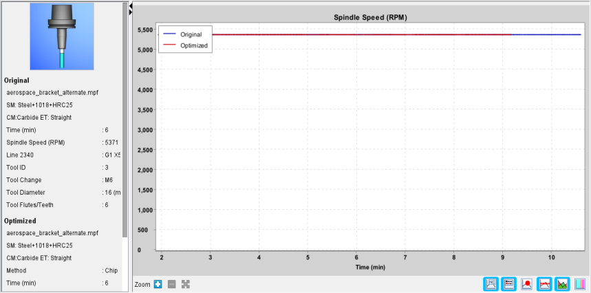
Spindle Speed — This chat displays the spindle speed.
Milling — Spindle speed of the tool for the associated subinterval of motion.
Turning — Spindle speed of the cut stock spindle for the associated subinterval of motion.
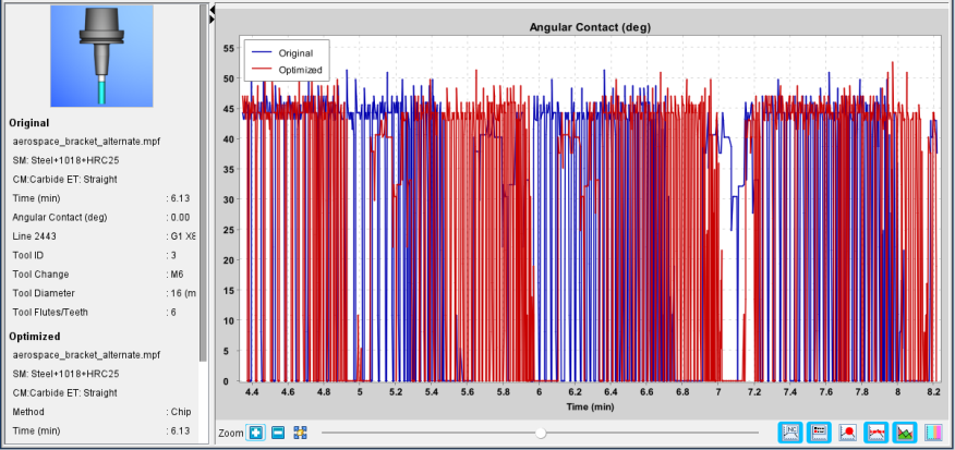
Angular Contact — This graph displays the time the tool is spent in contact with the material while at an angle.
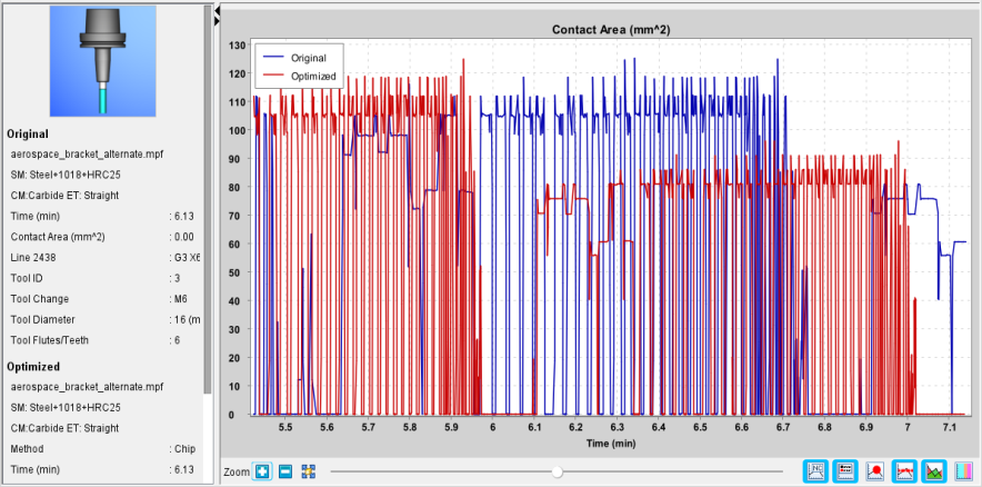
Contact Area — This graph displays the area of the tool that is in contact with the material.
Milling — The surface area of the portion of the tool in contact with material for the associated subinterval of motion. For this calculation, the tool is treated as a solid body-of-revolution making contact area with material.
Turning — The area of the profile of removed material in the turning plane for the associated subinterval of motion. Interrupted cuts have no impact on this value. It is the idealized turning profile result.
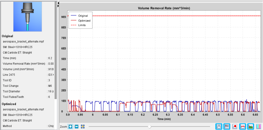
Volume Removal Rate — This graph displays the volumetric material removal rate of the tool.
Milling — The volumetric material removal rate of the tool for the associated subinterval of motion. Calculated as the volume of material removed during the motion divided by the time the motion took.
Turning — The volumetric material removal rate of the tool for the associated subinterval of motion. Calculated as the volume of material removed during the motion divided by the time the motion took. The volume value used is the change in turning volume of the idealized spun cut stock meaning interrupted cuts will not be reflected in this value.
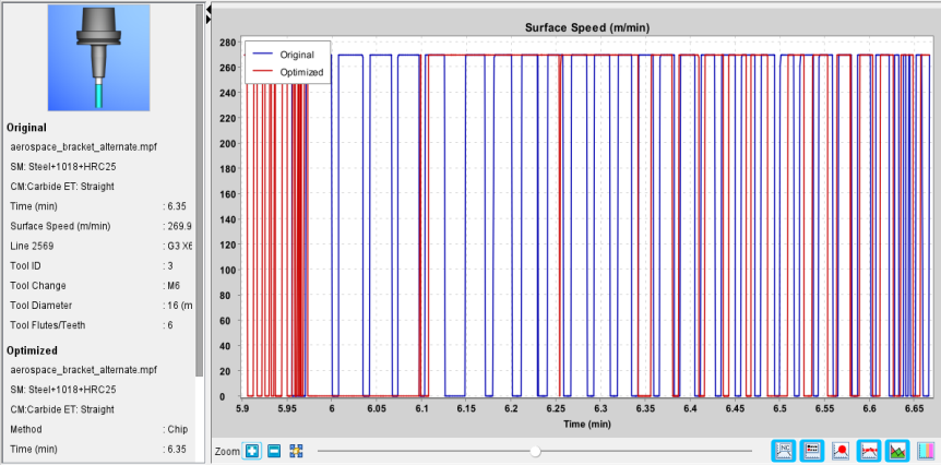
Surface Speed — This graph displays the maximum surface speed anywhere across the entire tool engagement.
Milling — The maximum value of the surface speed of a cutting edge anywhere in material contact for the associated subinterval of motion. This maximum value is a function of Spindle Speed and the maximum radius of material contact on the tool from the spindle axis.
Turning — The maximum value of the surface speed of a cutting edge anywhere in material contact for the associated subinterval of motion. This maximum value is a function of Spindle Speed and the maximum radius of material contact on the tool from the spindle axis.
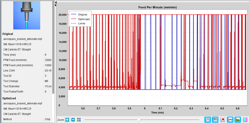
Feed Per Minute — This graph displays the feed per minute feedrate.
Milling — The feed per minute feedrate of the tool for the associated subinterval of motion.
Turning — The feed per minute feedrate of the tool for the associated subinterval of motion.
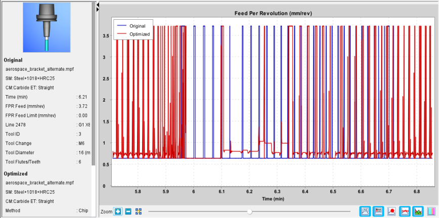
Feed Per Revolution — This graph displays the feed per revolution feedrate.
Milling — The feed per revolution feedrate of the tool for the associated subinterval of motion.
Turning — The feed per revolution feedrate of the tool for the associated subinterval of motion.
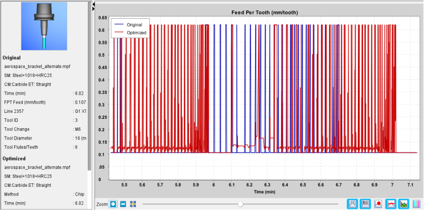
Feed Per Tooth — This graph displays the feed per tooth feedrate.
Milling — The feed per tooth per revolution feedrate of the tool for the associated subinterval of motion.
Turning — The concept of teeth does not apply to turning. In calculations, turning is implicitly treated as having one tooth. Therefore, this value is equal to Feed Per Revolution.
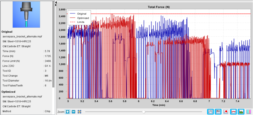
Total Force — This graph displays the total cutting force acting on the tool.
Milling — The maximum value of the total cutting force acting on the tool at any point throughout the associated subinterval of motion. Milling is a dynamic process in which the instantaneous cutting force changes continuously as the tool rotates. The returned value is the maximum of all these instantaneous force values.
Turning — The maximum value of the total cutting force acting on the tool at any point throughout the associated subinterval of motion.
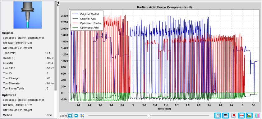
Radial/Axial Force — This graph displays the radial and axial force acting on the tool.
Milling — The Force value decomposed in the radial and axial directions of the tool. The radial value is always positive. The axial value is signed with positive values acting on the tool in the positive (upward) direction of the tool.
Turning — The Force value decomposed in the radial and axial directions of the spindle. The radial value is always positive. The radial value is the sum of all non-axial forces. This means that when viewed from a turning plane decomposition perspective, it is the combination of both the radial and normal forces acting on the tool. The axial value is signed with positive values acting on the tool in the positive direction of the spindle.
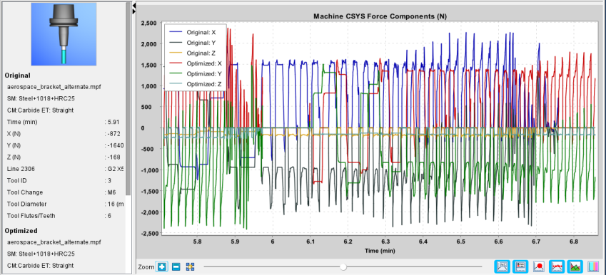
Machine Force — This graph displays the force acting on the tool expressed in the machine coordinate system.
Milling — The Force value decomposed into the Machine CSYS.
Turning — The Force value decomposed into the Machine CSYS.
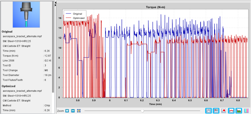
Torque — This graph displays the torque acting on the spindle.
Milling — The maximum value of the total cutting torque acting on the tool at any point throughout the associated subinterval of motion. Milling is a dynamic process in which the instantaneous cutting torque changes continuously as the tool rotates. The returned value is the maximum of all these instantaneous torque values. This value is unsigned and always positive.
Turning — The maximum value of the total cutting torque acting on the tool at any point throughout the associated subinterval of motion. This value is unsigned and always positive.
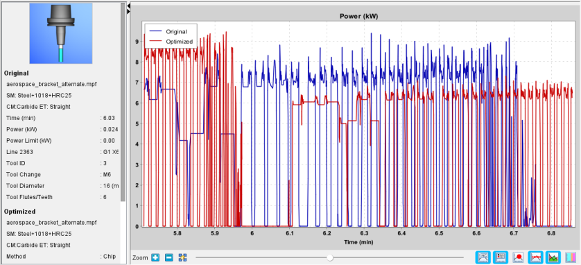
Power — This graph displays the power used to drive the spindle.
Milling — The maximum value of the total cutting power exerted by the tool at any point throughout the associated subinterval of motion. Milling is a dynamic process in which the instantaneous cutting power changes continuously as the tool rotates. The returned value is the maximum of all these instantaneous power values.
Turning — The maximum value of the total cutting power exerted by the tool at any point throughout the associated subinterval of motion.
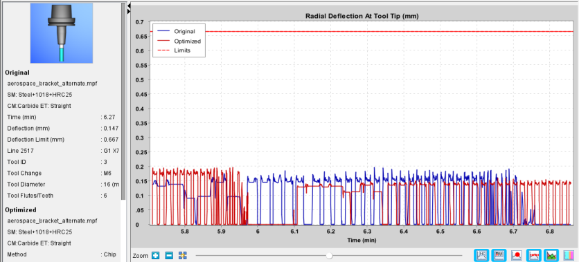
Deflection — This graph displays the radial deflection at the tip of the tool.
Milling — The maximum value of the radial deflection of the tool tip at any point throughout the associated subinterval of motion.
Turning — Deflection is not supported for turning.
RMB
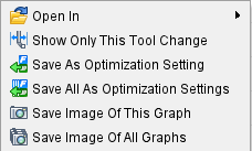
When right-clicking within the display area, the following menu options are available:
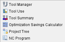
Open in — Generates a menu of options to view the selected tool. Options where to open include Tool Manager, Tool Use, Tool Summary, Optimization Savings Calculator, Project Tree, and NC Program.
Show Only This Tool Change — Displays only the selected tool change in the graphs.
Save As Optimization Setting — Saves only the value on the graph where you right-clicked.
Save As All Optimization Setting — Saves all applicable optimization values (Maximum Chip Thickness, Total Force, Power, and Radial Deflection At Tool Tip)
Save Image of This Graph — Saves an image of the selected graph.
Save Image of All Graphs — Save a combined image of all the displayed graphs.
Zoom features

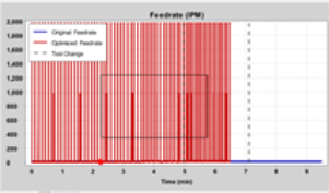
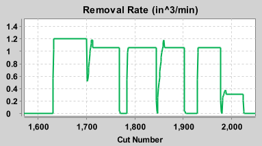
X Axis Zoom — The X Axis Zoom feature enables you zoom in or zoom out along the X Axis of the graph. You can also zoom to a box by drawing a bounding box with the mouse while holding down the right mouse button.
Example:
| Draw the bounding box | Zoomed in to bounding box |
|---|---|
 |
 |
 (X Axis Zoom In) — Use this icon to incrementally “zoom in” on the graph along the X axis. You can also use the CTRL key + scrolling up with the mouse wheel to zoom in.
💡 Tip: After zooming in, use the mouse thumb wheel up/down function to scroll left/right respectively along the zoomed-in portion of the graph
 (X Axis Zoom Out)— Use this icon to incrementally zoom out on the graph along the X axis. You can also use the CTRL key + scrolling down with the mouse wheel to zoom out. This option is naturally grayed out until Zoom In has been used at least once.
 (X Axis Fit) — Use this icon to “fit” the entire graph along the X axis into the window.
Slide bar — You can use the slide bar to control your location in the graph. Moving the slider to the left moves you towards the beginning of the chart and moving the slider to the right moves you towards the end of the chart. The slide bar only appears after Zoom In has been used first.
💡 Tips:
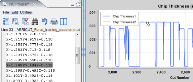
If the NC Program panel is displayed, you can click on a specific point along the graph and the corresponding line in the NC program will become highlighted as shown in the picture below.
Bottom Toolbar
The features on the bottom toolbar can be toggled on (highlighted) or off (not highlighted) to activate various display options.
 NC Program Click — When this option is toggled on (highlighted), clicking the graph will bring up the NC program corresponding to the graph and highlight the line of code that matches the X position of the graph. This function is only enabled when a single file is being displayed or if it is determined that all of the filed being displayed are related to one another or come from the same NC program. The “NC Program” window must be open for the line to be highlighted.
 Legends — When this option is toggled on (highlighted), the graph will display a legend which explains which color line corresponds to which data of the graph.
 Mouse Followers — When this option is toggled on (highlighted), the graph will display a bright red dot (or multiple bright red dots depending on if Original and Optimized NC Programs are toggled on and which graphs are selected) that follows the horizontal movements of your mouse. Wherever the dot lands, that portion of the graph will be used to generate the Data Display.
 Optimization Limits — When this option is toggled on (highlighted), the graphs will display a horizontal dashed or dotted line indicating a limit value that has been specified in Tool Manager. The limit line enables you to more easily visualize where tool force spikes are occurring.
 Fill Comparison — This feature displays total time of the selected/hovered tool change for every file that is loaded, displays the Time Savings percent between optimized and original files, and will only appear when there is a valid comparison state (i.e. only one file is being displayed or more than one file is being displayed but the graphs are not set to "Subinterval" for the X axis option).
 Cut Colors — This feature applies each tool’s cut color to graph backgrounds.
Graphs Data Display
The Graphs Data Display appears on the left hand side of the Graphs window.
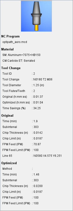
Graphs window when using NC Program Review Mode
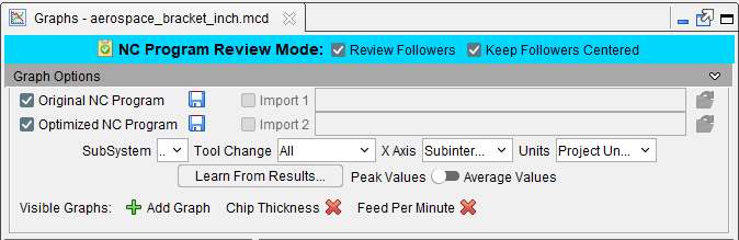
NC Program Review Mode — When NC Program Review is started in the simulation, Graphs will enter into NC Program Review Mode where it follows along with the review. A follower dot shows where on the graphs the current review position corresponds to. The Data Display will display the data for this review position if the mouse if off of the graphs, or the mouse value if the mouse is over the graphs. Graphs NC Program Review Mode is automatically ended when NC Program Review is ended in the simulation.
Review Followers — When this option is toggled on (checked), the graph will display a cyan dot (or multiple cyan dots depending on if Original and Optimized NC Programs are toggled on and which Graphs are selected) that follows the current position of the NC Program Review. Wherever the dot lands, that portion of the graph will be used to generate the Data Display (when the mouse is not over the graphs).
Keep Followers Centered — When this option is toggled on (checked), the graph view will automatically center about the Review Follower position any time the follower(s) moves. This is useful when zoomed in on the graphs and the NC Program Review is being played or stepped.